Theory

Radial Basis Functions are first introduced in the solution of the real multivariable interpolation problems. Broomhead and Lowe (1988), and Moody and Darken (1989) were the first to exploit the use of radial basis functions in the design of neural networks.

The structure of an RBF networks in its most basic form involves three entirely different layers: an input layer, a hidden layer with a non-linear RBF activation function and an output layer with linear activation functions.

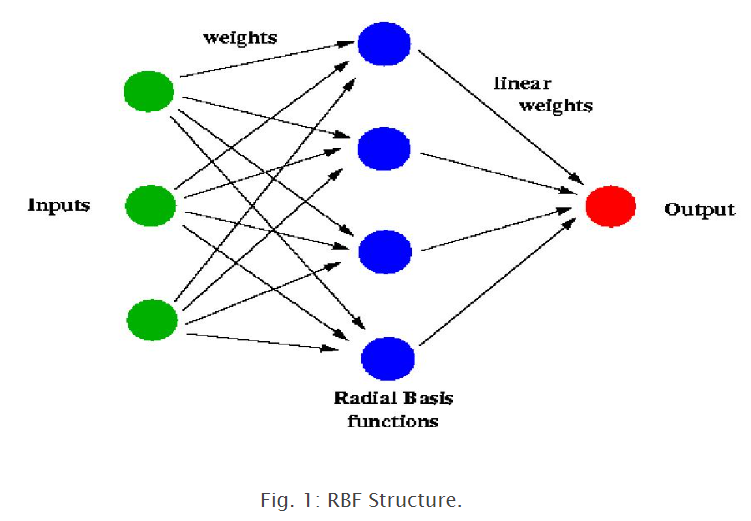
Input Layer: The input layer is made up of source nodes (sensory units) whose number is equal to the dimension of the input vector.

Hidden Layer: The second layer is the hidden layer which is composed of nonlinear units that are connected directly to all of the nodes in the input layer. It is of high enough dimension, which serves a different purpose from that in a multilayer perceptron. Each hidden unit takes its input from all the nodes at the components at the input layer. As mentioned above the hidden units contains a basis function, which has the parameters center and width. The center of the basis function for a node i at the hidden layer is a vector c_i whose size is the as the input vector u and there is normally a different center for each unit in the network. First, the radial distance d_i, between the input vector u and the center of the basis function c_i is computed for each unit i in the hidden layer using the Eucledian distance:

$$ \begin{align*} d_i &= ||u - c_i|| \ \end{align*} $$

The output h_i of each hidden unit i is then computed by applying the basis function G to this distance:

$$ \begin{align*} h_i &= G(d_i, σ_i) \ \end{align*} $$

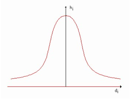
As it is shown in Figure 2, the basis function is a curve (typically a Gaussian function, the width corresponding to the variance, σ_i) which has a peak at zero distance and it decreases as the distance from the center increases.

Output Layer: The transformation from the input space to the hidden unit space is nonlinear, whereas the transformation to the hidden unit space to the output space is linear. The j^th output is computed as:

$$ \begin{align*} x_j &= f_j(u) &= w_{0j} &+ \sum_{i=1}^{L} (w_{ij}h_i) &&&&&& j = 1,2,3,....,M\ \end{align*} $$

Mathematical Model:In summary, the mathematical model of the RBF network can be expressed as:

$$ \begin{align*} x &= f(u), f:R^N \to R^M\ \end{align*} $$

$$ \begin{align*} x_j &= f_j(u) &= w_{0j} &+ \sum_{i=1}^{L} (w_{ij}G(||u - c_i||)) &&&&&& j=1,2,3,.....,M\ \end{align*} $$

where d_i is the the Euclidean distance between u and c_i.